Since this is a theoretical study, Food web dynamics was based on a generalized Rosenzweig-MacArthur model with stochastic parameters with functional response type II and III.

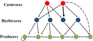
The model communities consisted of triangular shaped food web (fig 1), which means the number of species decrease with the increasing trophic level. The food web model was constructed with three trophic levels; basal species (primary producers), herbivores (primary consumers), and carnivores (secondary consumers). Some carnivore species were also omnivores preying on both primary consumers and primary producers. In this study, food webs with 6, 12, 18 and 24 species was used. A six species web had three basal species, two herbivores, one carnivore and this proportion of species at the different trophic levels was kept constant in webs of different sizes. In each food web, four different connectances (C); 0.07, 0.14, 0.21 and 0.28 were used ( C= L/S² where L is the number of interaction link between consumer and producer species and S is the number of species in that particular food web).

Species growth (mortality) was constructed as the function of temperature sensitivity and temperature standard deviation.

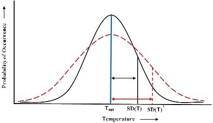
Figure 2 illustrates the temperature variability with the probability of occurrence of weather event in y-axis and temperature in x-axis. The temperature data used in this model was based on the daily recorded atmospheric temperature of Uppsala from year 1722 to 2010 from Swedish Meteorological and Hydrological Institute (SMHI) (Bergström & Moberg 2002).Topt is the optimum temperature, SD(T) is the temperature standard deviation and SD(T)ˈ is the increased temperature standard deviation. When the SD(T)ˈ increases the normal distribution curve becomes more flat resulting in higher possibility of occurrence of extreme weather events and larger effect on growth /mortality rate.

Figure 3: Panel A and B shows the tolerance curve of temperate and tropical species based on empirical studies respectively (Deutsch et al. 2008). Panel C illustrates the symmetrical tolerance curve which is used to create the model for this study. The sensitivity k determines the steepness of the curve. If the value of k is small then tolerance is high and the curve is wider (less steep) and if the value of k is larger (i.e kˈ) then tolerance is low and the curve is narrower (steeper). T_opt is the temperature where, the intrinsic growth (mortality) rate (b_opt) of the species is maximum (minimum). CT_min and CT_max is the minimum and maximum tolerance temperature respectively where fitness of an individual species is zero.