Department of Physics, Chemistry and Biology (IFM)

In this study I used the gut content dataset which  was sourced from; https://access.afsc.noaa.gov/REEM/WebDietData/DietDataIntro.php . With regards to climatic conditions for Eastern Bering sea, an already classified temperature was used. This included the following classified temperate regimes; warm years  included 2001-2005 & 2014-2016; Cold years included 2006-2013.

Analyses

1. Calculated food web metrics for each food web

Based on the classified temperature mentioned about separated into two food web namely warm and cold. Using these two food webs I calculated  species richness (the total number of species in a food web), connectance (the proportion of potential links among species that are actually realized and expressed as C = L/S² (where L is the feeding interactions and S are species), average generality (average number of links to prey species) and average vulnerability (average number of links to predators) for each web.  I also calculated  dissimilarity in species composition between the cold and the warm food web using; 

          2. Compared the results for (1) between the two food web to assess potential changes

          3. Using the functional group model to establish the groups in each food web

I used the group model described by (Allesina and Pascual 2009), and the approach is as follows; firstly, one should consider a food web as a network N which is made of S nodes and L links between the nodes, where S represent species or a collection of similar species and L the directed connections representing the consumer–resource interactions. The network can be described as a matrix – an adjacency matrix, in which each coefficient a_ij is 1 if species j interacts with species i, and 0 if otherwise. If one wants to reproduce an empirical network N with the simplest random process that would be connecting each node with any other node with a probability p, and not connecting with probability (1-p). A network N with S nodes and L interactions where the interactions are defined by a random process with fixed interaction probabilities is a directed random graph (Erdös and Rényi 1960), and  the probability of producing exactly N is:

The goal with the group model is to divide the species into relevant groups and as such the probabilities will refer to probability of connecting one group of species to any other group of species. Allesina and Pascual, ( 2009) gives an illustrative example of a network where the nodes have been divided into two groups. This study did reproduce their example here. Where  equation (2) is modified by dividing the nodes into two groups (r and g), which gives four probabilities for connections:

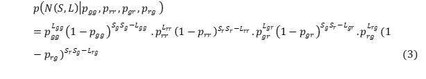
where is the probability of connecting a node in group x with a node in group y,  is the number of links connecting nodes belonging to group X to nodes belonging to group Y, and S_x is the number of nodes in group X. This equation can then be generalized to an arbitrary number of groups k:

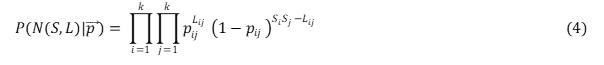
The vector p contains all the probabilities p_ij . If each node is assigned to a group of its own (that is they will have S number of groups in the network),  Each probability is then set to either to 0 or 1, and the process will therefore always produce exactly the empirical network (N)  - the probability of recovering the data is 1  (Allesina and Pascual 2009), but this is not very informative. If one wants to find the best grouping of the species in the network N, one needs to search over all possible ways of combining the species and preform model selection. Following the approach in (Sander et al. 2015), this study compared the marginal likelihoods of the different groupings. As there is an extensive number of possible groupings to test, Metropolis-Coupled Markov Chain Monte Carlo (MC³)  with a Gibbs sampler was used to find the optimal grouping.

Using the above described group model, the functional groups were established both  in the cold and warm years respectively.  The model was executed in C and to obtain the optimal grouping for each temperature regime,  20 runs was done using MCMC following the procedure in Sander et al. (2015) with 200000 steps per data sets.  The results (groups identified by the model) was used to interpret if there were any potential changes between the two temperature regimes using ecological properties. The following metrics were calculated;

1. The total number of species that changed groups between the two regimes
2. Determined a group to be the same group between the two regimes if it contained 80% of the species belonging to that group and maintained the same group between the two regimes
3. Looked at the distribution of the taxonomic phyla and variation in phyla composition in the different groups between the two regimes. 
4. Compared  the variations in phyla diversity and composition in the different groups between the cold and warm regimes.