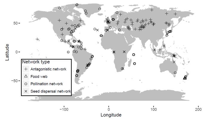
I used 250 ecological networks from previous studies, differentiated into food webs, bipartite mutualistic webs and bipartite antagonistic webs. Bipartite mutualistic webs were further split into plant-pollinator and seed dispersal networks. All networks were then attributed with spatial information (Figure 1), including coordinates, altitude and 7 land cover classification. Climate data was also added for all networks, including annual mean temperature, annual temperature range, annual precipitation, and precipitation seasonality. Since most climate data was based on terrestrial measurements, marine networks were excluded from the study. Additionally, historical temperature and precipitation change velocities since the last glacial maximum (21 000 b.p.) were added for each network.

Generality and vulnerability shows the average specialisation for predators and prey in a network. However, it does not describe whether specialisation is highly concentrated in a few species or evenly distributed. To get a measurement of the distribution, I calculated the generality and vulnerability of each species in the networks. From these values, I calculated the width between quantiles 1-3 and divided with the maximum generality/vulnerability for each network.

Intervality was analysed from both predator (or equivalent in pollinator, seed dispersal and antagonsitic networks) and prey perspective for each network. Finding the most interval ordering consists in organising the species in a way that minimises the discontinuity in all species interactions. For each network, the most optimal interval ordering was searched for using a stochastic approach with 100 iterations. Following this, 100 random orderings were made to get a relative comparison with fully randomised gaps. While higher numbers of permutations could have been desirable, they were limited to 100 due to heavy computational requirements. The randomised orderings were compared to the previously obtained optimum to obtain a comparison to a randomised network relative to it's own size. A more negative value means that networks are more interval (having fewer gaps than a randomised ordering).

Dimensionality uses an approach similar to intervality with ordering species on hypothetical trait-axes based on their interactions. The principal for the dimensionality analysis starts with estimating the upper limit of dimensions. Species interactions are then analysed for the different number of potential dimensions, obtaining the narrowest interval of each axis which encompasses prey or predators. If there are species within these intervals which lack interactions, this means that additional dimension(s) are necessary to explain the interactions. This is done for all species in the networks from both predator and prey perspectives, from which finally the minimum number of dimensions can be obtained.

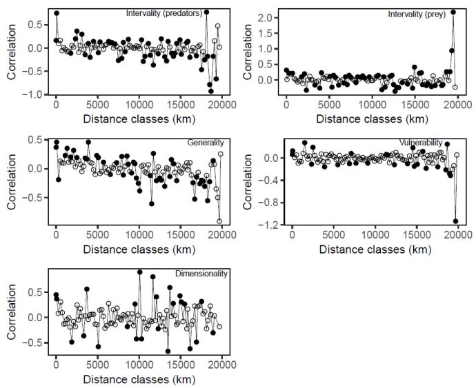
Spatial autocorrelation can be described as pairs of observation more similar (positive autocorrelation), or less similar (negative autocorrelation) based on their proximity, when compared to randomly picked values. From a biological point of view, this is of course an expected and common property. From a statistical point of view however, it may be more troublesome. A general requirement in most significance tests is that the data is normally distributed and that errors are independent with constant variance. Spatial autocorrelation breaks these rules, making regular approaches unreliable.

I tested all my response variables for spatial autocorrelation using coordinate based spatial correlograms. While many points indicated spatial autocorrelation, the mixture between positive and negative autocorrelation rule out any real autocorrelation (Figure 2). Without any spatial autocorrelation patterns detected, there was no reason to consider any further actions regarding this.

Selecting models, or "best models", for all combinations of networks and variables can be both tedious and erroneous. Instead, I used a model averaging approach of top model sets. With this approach, first variables were split into geographical and environmental categories. For each combination of network type and response, I then created separate global models for each respective variable type. I included interactions, but restricted interactions to within the geographical or environmental (contemporary or historical) categories. Additionally, I only included two-way interactions. This was done out of practical reasons, as the model averaging function used is restricted to maximum 30 factors (including interactions), as well as for simplifying the interpretation of the results.

The global models were standardised by centring and dividing by two standard deviations. From the global models, I then created nested model sets, meaning separate models with all different combinations of variables. Linear regressions were made for each model, which were given certain weights. The weights are based on an information criterion, which scores based on correlation, but penalises over-fitting (including more factors).

For model averaging, including either too many and too few extracted models can be detrimental for the results. Thus, I created appropriate subsets of the top models based on their information criterion scores. These top model sets were then averaged while using the weights of the included models. Estimates, confidence intervals and relative importances of the factors were used to present the results. Confidence intervals not overlapping zero have a significant effect. The relative importance of the different factors indicates the overall weight of top models they are present in.