It is generally accepted that biodiversity follows a latitudinal diversity gradient (LDG), with biodiversity increasing with the proximity to the equator. The LDG is not limited to specific types of organisms or environments, but not without exceptions, e.g. conifers and crayfish. Environmental factors are closely linked to the LDG, including both contemporary and historical factors, such as temperature, precipitation, and long term climate stability. How and why these factors affect ecosystems to enable higher biodiversity instead of just increasing overall biomass are however not fully explored, but differences in how species interact with each other may play an important part.

Species interactions in ecosystems largely depend on practical biological attributes, or traits. E.g., a predator may be physically restricted to prey of certain intervals of body size and mobility. Differences in occupancy of various trait axes can be seen as the basis of niches. Subtle differences may also explain coexistence of species, allowing a higher biodiversity, such as the niche breadth (e.g. species targeting certain range of body size) being narrower at lower latitudes.

Ecological networks are good tools in understanding these interactions, and making predictions of perturbations. Essentially, an ecological network shows which species are included in an ecosystem, and their interactions. Networks may consist of complete ecosystems or, certain subnetworks of specific species groups. Classically, the networks are represented as food webs with multiple trophic levels with predator-prey interactions, or bipartite networks, which are restricted to two trophic levels. Bipartite networks are often further divided into either mutualistic (e.g. plant-pollinator or seed dispersal interactions) or antagonistic (typically host-parasite interactions) networks. Various analyses can be applied, e.g. investigating complexity and stability, making predictions for perturbations, and making risk models. Understanding patterns and mechanisms behind differences in structure and function of these networks is a natural step in increasing knowledge and the accuracy of future ecological network models.

Network complexity can be analysed in many different ways. One of the most basic measurements is network connectance, which is the average number of links per species squared in a network. Generality and vulnerability are two measurements which expand this slightly. Here, the number of prey species (generality) or the number of predator species (vulnerability) of each species in a network is analysed. This gives an estimate of how specialised predators and prey are in networks. However, it does not catch variation between species within the networks. Hence, the difference between a network with some highly specialised and some extreme generalist species, and a network where all species are similarly specialised, is not necessarily detected.

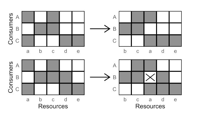
Another way to analyse network complexity is to look for how many different traits are required explain all interactions in a network. In this study, I use two different trait-based complexity metrics, intervality and dimensionality. Both metrics have a rather abstract way of looking at traits however, and have their basis in ordering species based on their interactions (Figure 1). By doing this, you can get a value on how close the interactions in an ecological network are to being dependant on a single traits (intervality), or how many traits are required to explain all interactions in a network (dimensionality). Given the aspect of the LDG, it is reasonable to assume that higher dimensionality (more traits) and lower intervality (less similar to a one-trait network) would follow the same gradient, as they would in principle open opportunities for more niches, explaining the diversity gradient.

Here, using the network metrics intervality, dimensionality, generality and vulnerability, I analyse how network complexity varies with geographical and environmental factors for different network types. The aim is to evaluate global patterns and important factors to include when making future models and predictions.