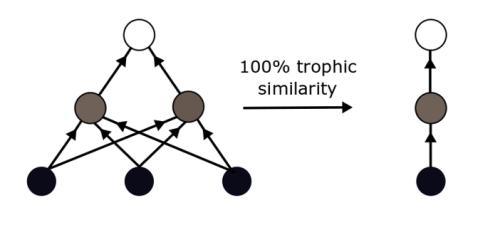
In the first set of analyses I tested the effects of aggregating species based on their trophic similarity. Trophic similarity is the proportion of shared predator and prey between species. 

I created a series of increasingly aggregated networks using hierarchical clustering. Hierarchical clustering identifies homogeneous groups of species based on their trophic similarity. All species started as separate nodes and were combined with the most similar node until there was only one node left. More similar nodes are clustered first, yielding a "tree" of increasingly merged nodes. 

To create each aggregated network, I combined species in the meta-network with trophic similarities above a given threshold. I used thresholds of 1.0, 0.9, 0.8, 0.7, 0.6, 0.5, 0.4, 0.3, 0.2, and 0.1 to create increasingly poorly-resolved and highly-aggregated network. 

I used two types of clustering methods for the hierarchical clustering: complete linkage and single linkage. The complete linkage method requires all species in an aggregated node to have the specified threshold to all other species. The single linkage method require species to have the specified threshold with only one other species in an aggregated node for them to all be linked. This means that the single method tends to give fewer and larger aggregated nodes than the complete method.

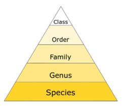
Species with similar taxonomies are often grouped in poorly-resolved food webs. To simulate this, in the second set of analyses I aggregated species within taxonomic groups. I clustered taxa to several taxonomic levels: from species (in the original web) to genus, family and class, creating an aggregated network at each level. The species were not clustered further to phylum or kingdom level to make sure there were enough nodes remaining in the aggregated  web to form at least one motif. 

For trophic and taxonomic aggregation, links between aggregated nodes were assigned using several different criteria. I selected linkage criteria so as to obtain the largest possible range of connectedness.  The strictest criterion was the minimum-linkage criterion, where all members of node A must interact with all members of node B in order for the two nodes to be linked. 

In the weakest criterion, the maximum-linkage criterion, two nodes were linked if at least one of the members of node A has a link to at least one member of node B. 

Between these two criteria is the average-linkage criterion, which required at least half the species in node A to interact with at least half the species in node B for them to be linked. 

To fill the gaps between the other three criteria, I used intermediate linkage criteria that were similar to the average-linkage criterion except requiring 75 % or 25 % of the species in node A to interact with at least 75 % or 25 % in node B for them to be linked. 

 After assigning links, there was no connection between the nodes in the network compiled in the trophic similarity aggregation using single method with the similarity coefficient of 0.10. This result was equivalent for all linkage methods. This lead to a problem due to no motifs could be created. This network were therefore excluded from further analyses.

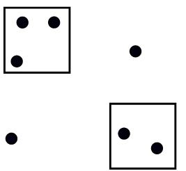
In the third aggregation, I was interested in the effects of spatial scale on motif frequencies rather than the effects of resolution of nodes within the networks. When compiling networks the constrains of spatial boundaries might result in an ignorance of variability. Species and links can be missed. Aggregation is therefore used in some studies.

I used the 32 subwebs to simulate the effects of spatial scale. To create a series of webs describing the Baltic Sea at different spatial scales, I combined subwebs based on the distance between them, ending with the meta-network describing the entire Baltic Sea.

Neighbouring sites were aggregated using hierarchical clustering based on the distances between them, starting with a threshold of  100 km and increasing by 100 km at each step until only one meta-network of the entire Baltic Sea was left. I used, just as in the aggregation bassed on trophic similarity, two types of clustering methods for the hierarchical clustering.

Distances between networks were calculated from their coordinates by estimating the shortest distance between two points on an ellipsoid. 

Unlike trophically or taxonomically-aggregated webs, spatially-aggregated webs gained species and links with increasing aggregation.

To quantify the structure of each aggregated network, I calculated the frequencies of each three-species motif on each network. The frequencies of motifs were quantified as normalised frequencies. Normalised frequency are calculated by dividing the count of each motif by the total of all motifs in the network.   

After determining the frequencies of motifs in each aggregated web, I wanted to test if networks with more different levels of resolution have more different structures.

First I calculated differences between motif frequencies in the aggregated webs using Bray-Curtis dissimilarity. I chose to use Bray-Curtis dissimilarity because it is a robust measurement for ecological questions, only measuring differences between networks based on positions were at least one of the networks have a frequency not equal to 0. Therefore, two networks with shared zeros will not appear more similar

I then used a Mantel test to see if there is a correlation between dissimilarity of motif frequencies and change in resolution. The Mantel test evaluates correlation between two distance matrices, through permutations of the rows and columns in one of the matrices.